Number Formatting

While working with number values in Webix SpreadSheet, you have two options of setting format for them:

• make use of the provided default formats with the possibilities to adjust them to your needs
• create a custom format that will meet your requirements

Default Number Formats

The following default formats for numbers are available:

• Common - no formatting applied
• Currency - a format to display a number as currency
• Number - a format to display a number with delimited tens, hundreds and thousands
• Percent - a format to display a number as percentage (%)
• Date - a format to display a number as date
• Text - a format to display a number as string

The default formats can be customized via the dedicated interface:

Related sample:  Number Format

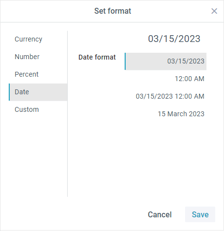
Decimal places

You can increase/decrease decimal places via the corresponding API method changeDecimals.

To apply the method to one cell, call the method with the following parameters:

• row - (number) the row ID
• column - (number) the column ID
• change - (number) the number of decimal places to be added (if the number is positive) or deleted (if the number is negative)
• page - (string) optional, the name of the sheet

// add 3 decimal places for the value of the cell C3
$$("ss1").changeDecimals(3, 3, 3, "Sheet1");

The method also works for a range of cells. Use the parameters below:

• first - (object) the row and column numbers of the first cell in a range
• last - (object) the row and column numbers of the last cell in a range
• change - (number) the number of decimal places to be added (if the number is positive) or deleted (if the number is negative)
• page - (string) optional, the name of the sheet

// delete 2 decimal places for values of cells in the range C3:E5
$$("ss1").changeDecimals({row:3, column:3}, {row:5, column:5}, -2, "Sheet1");

Custom Number Format

It is also possible to apply a custom format of displaying a numeric value to a cell or a selected range of cells.

There is a handy interface for setting a custom number format:

Related sample:  Number Format

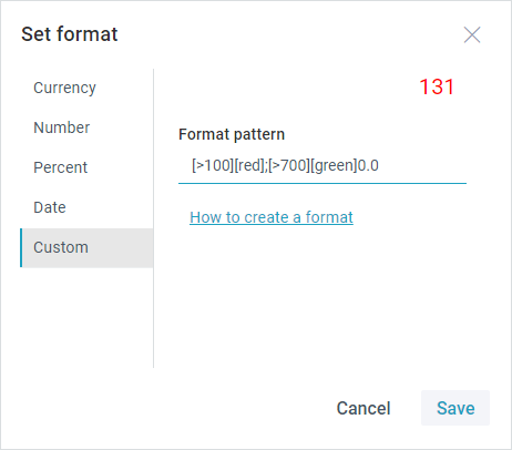
Custom format structure

A custom format notation presents a string which consists of several code sections, separated by semicolons.

Each code section may include:

• [condition] in square brackets - e.g. [>1000], to compare the cell value with
• [color] in square brackets - e.g. [blue]
• format as a set of zeros (e.g. 0.0;) which:
  • are separated by decimal or thousand separators
  • have additional 0 after the separator to display insignificant zeros or # to ignore them
• text - e.g. Text, that should be displayed in this cell

For example:

"[>1000][red];[>100][green]0.0;[blue] Small"

Applying custom format

For setting a custom number format for a cell value, make use of the setFormat method. It takes three parameters:

• rowId - (number) the row id
• columnId - (number) the column id
• format - (string) a string with conditions for formatting the cell content. Each separated by semi-colons
• page - (string) optional, the name of the sheet

$$("ss1").setFormat(2, 2, "[>1000]>0.0;[>100]Check 0,000.0#;[=0]Nope", "Sheet1");

Specifying conditions

The condition should be enclosed in square brackets and consist of a comparison operator and a value. For example, the following format colors numbers that are less than or equal to 150 in green and numbers that are greater than 150 in orange.

"[<=150][green];[>150][orange]"

You can also apply conditional formats to cells (for example, highlighting a cell depending on its value).

Specifying colors

To specify the color for a section of the format, type the name of one of the available colors (green, red, blue, orange, black, violet or magenta) enclosed in square brackets in the section. The color code must be the second item in the section (after the condition).

Specifying significant digits, decimal and thousands separators

• 0 (zero) - the digit placeholder to display insignificant zeros, if a number has fewer digits than there are zeros in the format. For example, to display 4 as 4.0, use the format 0.0
• # - the digit placeholder to display only significant numbers (not to display extra zeros when the number has fewer digits than there are # symbols in the format)
• ? - works the same as 0 (zero), but adds a space for insignificant zeros on either side of the decimal point so that decimal points are aligned in the column
• . (period) - the digit placeholder to display the decimal point in a number
• , (comma) - the digit placeholder to display the thousands separator in a number

Localized delimiters

The decimal and thousands separators are taken from the applied locale. They can be redefined via the related properties of the i18n object as follows:

• decimalDelimiter

webix.i18n.decimalDelimiter = "'";
webix.i18n.setLocale();

• groupDelimiter

webix.i18n.groupDelimiter = "'";
webix.i18n.setLocale();

For prices:

• priceSettings:

webix.i18n.priceSettings = {
    groupDelimiter:" ", // a mark that divides numbers with many digits into groups
    decimalDelimiter:" "// the decimal delimiter
};
webix.i18n.setLocale();

Specifying position of a negative sign

The negative sign can be used at the beginning or end of a number: -577 or 577-. As an alternative, you can use parentheses around the number: (577).

The negative sign and its position are determined by the locale. They can be redefined using the following i18n object properties:

• minusPosition

webix.i18n.minusPosition = "after";
webix.i18n.setLocale();

• minusSign

webix.i18n.minusSign = "-";
webix.i18n.setLocale();

Styling Number Formatting

You can redefine the styling of default number formats via the corresponding CSS classes. There are three of them:

• webix_ssheet_format_int - for the Number format
• webix_ssheet_format_price - for the Currency format
• webix_ssheet_format_percent - for the Percent format
• webix_ssheet_format_date - for the Date format
• webix_ssheet_format_text - for the Text format

For example, the style of the Number format can be set as in:

<style>
    .webix_ssheet_format_int{
        color: blue;
        font-style: italic; 
    }
</style>

You will see the result in the number format dialog:

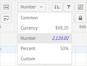
• webix_ssheet_format_{color} - can be used to specify styles for custom cell format

You can replace the last part of the class name, {color} with the name of the color which you want to use for formatting (green, red, blue, orange, black, violet or magenta) and apply the same word in the [color] section of the custom format.

For example, the default CSS style for the green color is the following:

<style>
    .webix_ssheet_format_green{
        color: green !important;
    }
</style>

And it is used in the custom format as follows:

"[>100][green]0.0"

Date Format

The default date format is mm/dd/yyyy.

The default format can be customized via the dedicated interface:

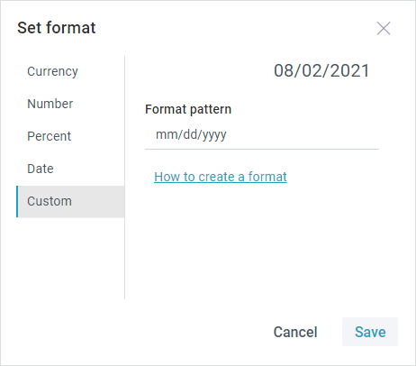
There are many built-in custom formats that user can enter into Format pattern field. For example, if you want to show the month name fully spelled out, you would use code mmmm. Here is a list of the custom date format codes and their result:

• m -3
• mm- 09
• mmm- Mar
• mmmm- March
• d - 1
• dd - 07
• ddd- sun
• dddd - Sunday
• y - 20
• yyyy - 2020

To change date color, define color section before the date code:

[violet]yyyy

Text Format

Text format is used to present numbers as a string.

The default text format looks as follow:

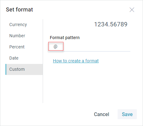
To change text color, define color section before the @ sign:

[red]@

Price Format

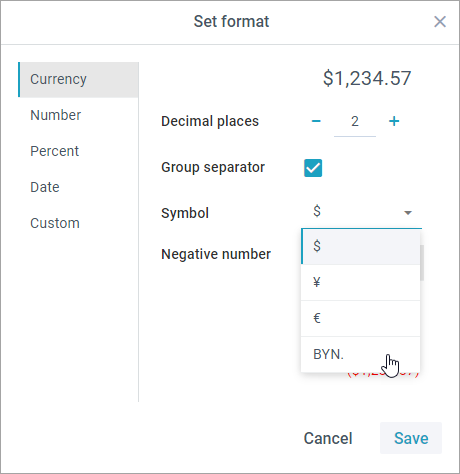
You can choose a currency symbol via the interface. By default, Spreadsheet offers 5 symbols: US dollar, Euro, Yuan, Portuguese real and Russian ruble.

To change this list, you can add an array of the desired marks to the current locale:

webix.i18n.spreadsheet.formats.currencies = [
    "{obj} ¥",
    "{obj} €",
    "{obj} BYN."
];

Related sample:  Spreadsheet: Custom Currency

Specifying position of a negative sign

Possible options for a negative sign position are:

• before - the negative sign before both the currency symbol and number: -£127.54
• inside - the negative sign before the number but behind the currency symbol: kr-127,54
• after - the negative sign after the number: €127,54-
• parentheses - enclosed in parentheses: ($127.54).

They can be redefined via the related properties of priceSettings object:

webix.i18n.priceSettings = {
    minusPosition:"before", 
    minusSign:"-", 
};
webix.i18n.setLocale();

Back to top