Using Formulas
SpreadSheet allows performing operations with simple cell content (numbers, strings) and operators (arithmetic, comparison, etc.) as well as with built-in functions and custom functions. It is also possible to combine regular operands and functions in more complex formulas. The component processes them and displays the result in the related cells.
Formula Syntax
The syntax of a formula is the same as in Excel.
- Formula must start from the '=' sign.
- The names of functions and cell references must be written in capital letters.
- The following elements can be used within formulas:
- basic mathematical operators: +, -, /, *, ^, % (the percent sign)
- comparison operators: <, >, <=, >=, <>, =
- the & operator for string concatenation
- numbers
- cell references
- Excel-like functions
"data": [
    [ 3, 2, "=A1+B2",""],
    [ 4, 2, "=7+8",""],
    [ 5, 2, "=7+B2",""],
    [ 6, 2, "=SUM(A3+D7)",""]
    ...
 ]
4 . There are two variants of recording a formula, both produce different results:
- if you want to apply a formula only to two certain cells, you need to specify comma-separated references to these cells, e.g.:
"data": [
 [ 7, 2, "=SUM(A3,D7)",""]
]
- if you want to calculate the values of cells in a range, you should define colon-separated references to the first and the last cells of the range, e.g.:
"data": [
 [ 7, 2, "=SUM(A3:D7)",""]
]
String Concatenation
You can concatenate string content of cells. There are three possible ways for this:
1 . the & operator with strings or cell references: "=nice"&"trip" or =A1&B2
2 . the + operator with same operands: ="nice"+"trip" or =A1+B2. The "+" operator behaves just as an ordinary JS addition operator (e.g. ="nice"+12).
You can also specify the strict mode for the "+" operation by setting the strict property to true. In this mode math calculations will behave similar to Excel:
// regular math
"1"+0 = 10
"a"+"b" = "ab"
// if `strict: true` is specified
"1"+0 = 1
"a"+"b" = #ERROR!
3 . apply the CONCATENATE() function, like this: =CONCATENATE("nice","trip" or A1,B2). It's also possible to connect strings from a range of cells to produce one continuous text: =CONCATENATE(C2:D4)
Using Named Ranges in Formulas
You can specify a name for a particular range of cells and then use it in formulas for calculations. Ranges can belong to a particular sheet or the whole Spreadsheet.
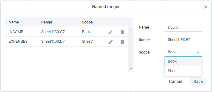
Thus, the formula will be easier to understand and work with.

Working with ranges via API
You can add a named range and manipulate it through the ranges module:
add()
Used to add new named range globally or to the active/specified sheet. The method takes the following parameters:
- name (string) - range name
- range (string) - range of cells to be included
- scope (string, boolean) - visibility scope.
- Pass a sheet name to add a range visible in this sheet only
- Pass true to add a range globally (visible throughout Spreadsheet).
To add a range to the active sheet, do not pass the 3rd parameter
// add "MYRANGE" range to Sheet 1
$$("ssheet").ranges.add("MYRANGE", "B2:C2", "Sheet 1");
Cross-references in Multiple Sheets
You can link data of several sheets and use these cross references in formulas to process them together.
The rules of creating a reference to an external sheet are quite simple:
- Sheet_Name!Cell_Name - to refer to a cell of other sheet, e.g. =Countries!A4
- Sheet_Name!Cells_Range - to refer to a range of cells from other sheet, e.g. =SUM(Countries!B2:B3)
- Sheet_Name!Named_Range - to refer to a named range from other sheet, e.g. =SUM(Countries!DATA)
Here are some use cases that show how to use cross references in multi sheets:
- provide reference to a cell from a different sheet, e.g. =Data!B8*D13 (where B8 is a cell from the "Data" sheet)
- fill a chart with data from a different sheet, e.g. =SPARKLINE(Countries!DATA,"splineArea","#6666FF") (where "DATA" is a named range from the "Countries" sheet)
- fill a dropdown with a data range from a different sheet, e.g. by referecning the range in the "Add dropdown" dialog as: Countries!NAMES (where "NAMES" is a named range from the "Countries" sheet)
Related sample: Spreadsheet: Multiple Sheets
Formula Editor
Spreadsheet possesses an advanced formula editor. Its main features are:
- providing the list of possible functions on entering the first letter of the function name in the input;
- entering formula operands either by selecting a range of cells or by typing in the cell reference.
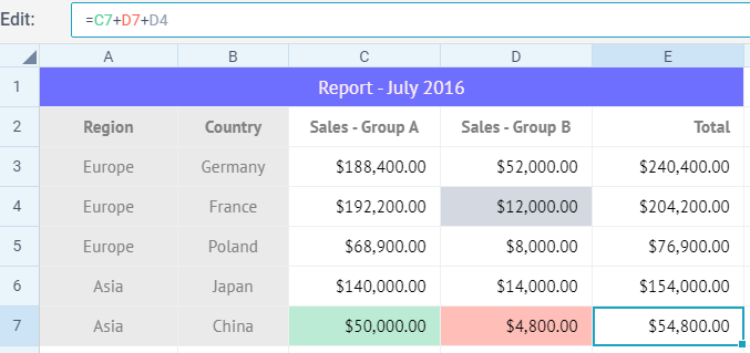
It's possible to disable the formula editor, just set the liveEditor property to false in the spreadsheet configuration:
webix.ui({
    view: "spreadsheet",
    data: base_data,
    liveEditor: false
});
Enabling math methods in the UI
Math methods are divided by categories: Common, Date, Text, Number, Financial. The Common math methods are available by default.
To enable math methods in the UI, you need to use the methods parameter and specify the category.
The methods parameter can be set as a string, e.g.: methods: "financial" or as an array, e.g.: methods:["number", "text"].
webix.ui({
    view:"spreadsheet",
    methods:["date", "text"],
    toolbar:"full",
    data:spreadsheet_data
});
To enable all the categories, use methods: "all". If the methods parameter is not specified, only the Common math methods are added to SpreadSheet.
You can search by category (note, that the Category field is hidden if the methods parameter is not specified):
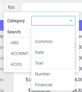
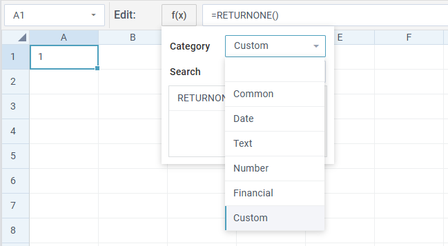
It is also possible to specify a custom category while adding a new math method:
webix.ui({
  view:"spreadsheet",
  id: "sheets",
  methods:"all",
  toolbar:"full",
});

webix.i18n.spreadsheet.liveEditor.custom = "Custom";
$$("sheets").registerMathMethod("returnone", () => 1, "custom");
$$("sheets").setCellValue(1, 1, "=RETURNONE()")
If you need to allow a custom method to generate HTML, while the xssSafe property is enabled, set the generateHTML parameter of the registerMathMethod() method to true. Check the example below:
const spreadsheet = webix.ui({
    view: "spreadsheet",
    xssSafe: true
});

spreadsheet.registerMathMethod("bold", v => `<b>${v}</b>`, null, true);
spreadsheet.setCellValue(1, 1, '=bold("text")');
Note that while using the method with allowed HTML generation in math formulas, you should specify only the method in the formula. For example: =IMAGE(...) will generate an image, but =IMAGE(...)&"text" will be escaped.
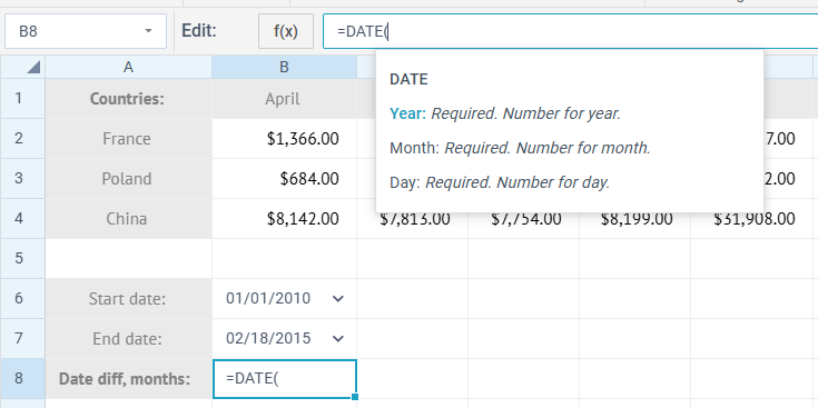
Tooltip for formula parameters
The formula editor is supplied with built-in suggestions for parameters of an entered formula. The suggestion contains a category of a math formula.
The tooltip with suggestions is available with the enabled liveEditor property.
Localizing parameters of formulas
The descriptions of the methods parameters are stored in the locale named webix.i18n.spreadsheet.liveEditor["functions-syntax"]. Thus you can translate them into the necessary language. The structure of methods in the locale is the following:
{
    methodName: [
        [parameter, description],
        ...
    ]
}
In case you have added your own method, you can add suggestions for its parameters by updating the locale.

Check the example below:
const ssheet = webix.ui({
  view:"spreadsheet",
  toolbar:"full"
});

ssheet.registerMathMethod("RANDOM", function(value){   value = value || 100;    return Math.round(Math.random()*value); });
webix.i18n.spreadsheet.liveEditor["functions-syntax"].RANDOM = [      ["Digit", "Optional. The number digit."]  ];
ssheet.setCellValue(1,1,"=RANDOM(100)")
Manipulating popup with formula parameters tooltip
You can reach the popup with suggestions for formula parameters using the following syntax: ssheet.$$("liveEditor").paramsPopup. For example, if you want to hide the tooltip popup, you can add a handler for the popup and return false from the callback function of the onBeforeShow event:
ssheet.$$("liveEditor").paramsPopup.attachEvent("onBeforeShow", ()=> false);
or simply remove all the methods from the locale:
webix.i18n.spreadsheet.liveEditor["functions-syntax"] = {};