Working with Cell Content

Locking/Unlocking Cells

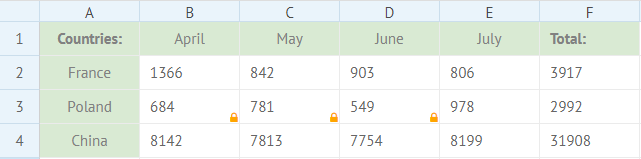
You can lock a cell or several cells to protect their content from editing. The locked cells will have a small yellow lock in the bottom right corner.

For this purpose, you need to use the lockCell method and pass three parameters to it:

• row - (number) the row ID
• column - (number) the column ID
• state - (boolean) true to lock a cell, false to unlock it
• page - (string) optional, the name of the sheet

// locks the cell at the intersection of the 3rd row and 2nd column
$$("ssheet").lockCell(3, 2, true, "Sheet1");

You can also lock/unlock several cells at a time with the lockCell method. Call it with different parameters:

• first - (object) the row and column numbers of the first cell in the range
• last - (object) the row and column numbers of the last cell in the range
• state - (boolean) true to lock a cell, false to unlock it

// locks 7 cells in the 2nd row
$$("ssheet").lockCell({ row:2, column:1 }, { row:2, column:7 }, true);
 
// locks 7 cells in the 2nd column
$$("ssheet").lockCell({ row:1, column:2 }, { row:7, column:2 }, true);
 
// locks 10 cells in the 1st and 2nd rows
$$("ssheet").lockCell({ row:1, column:1 }, { row:2, column:5 }, true);

In case the cell/cells to lock aren't specified, the method will lock the selected cell.

Related sample:  Lock cells

Changing the default styling of locked cells

You can modify the default styling of locked cells, by disabling yellow locks and applying some background color via CSS:

<style>
  .webix_lock:after{
    content:" ";
  }
  .webix_lock {
    background-color:#99f29d;
  }
</style>

Related sample:  Styling locked cells

Checking the state of a cell

You can check, whether a cell is locked, with the help of the isCellLocked method.

It takes two parameters:

• rowId - (number) the row id
• columnId - (number) the column id
• page - (string) optional, the name of the sheet

and returns true, if the cell is locked and false if it's unlocked.

var isLocked = $$("ssheet").isCellLocked(3, 2);

Adding an Editor into a Cell

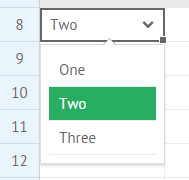
It's possible to add an editor into a cell of the sheet. It can include either some custom options or values of a cell range. You can also explicitly specify whether to add an empty option.

Use the setCellEditor to do it. The method expects three parameters:

• rowId - (number) the row id
• columnId - (number) the column id
• editorObject - (object) an object with two properties:
  • editor - (string) the editor type (ss_richselect, popup, excel_date, text)
  • options - (string,array) (the parameter is used if the editor is of the ss_richselect type) a range of cell references or an array of editor options
  • empty - (boolean) specifies whether to add an empty option
• page - (string) optional, the name of the sheet

$$("ss1").setCellEditor(8, 1, { 
    editor:"ss_richselect", 
    options:["One", "Two", "Three"] 
    }, "Sheet1");
 
// or
$$("ss1").setCellEditor(8, 2, { 
    editor:"ss_richselect", 
    options:"B3:B7", 
    empty:true 
    }, "Sheet1");

Getting the cell editor

You can get the editor set in a cell with the help of the getCellEditor method.

The method takes the following parameters:

• rowId - (number) the row id
• columnId - (number) the column id
• page - (string) optional, the name of the sheet

$$("ss1").getCellEditor(8, 1, "Sheet1");

It will return an object with two properties:

• editor - (string) the type of the editor (ss_richselect, popup, excel_date, text)
• options - (string,array) a range of cell references or an array of editor options

{ editor:"ss_richselect", options:["One","Two","Three"] }
 
// or
{ editor:"ss_richselect", options:"B3:B7" }

Related sample:  Dropdowns

Adding Checkboxes and Radio buttons into a Cell

You can add checkboxes and radio buttons into cells, mark them and check their states with the help of the corresponding SpreadSheet API methods.

To add checkboxes in a cell, use the addCheckbox method. To add radio buttons in a cell, use the addRadio method. Both methods take as a parameter an object with the start and end cells of the range to add checkboxes or radio buttons into:

• start - (object) an object with the start cell of the range set as {row:id, column:id}
• end - (object) an object with the end cell of the range set as {row:id, column:id}

$$("ssheet").addRadio({
    start:{row:1, column:1}, 
    end:{row:3, column:1}
});
 
$$("ssheet").addCheckbox({
    start:{row:1, column:3}, 
    end:{row:3, column:3}
});

Checking checkboxes and radio buttons

To mark a checkbox, apply the markCheckbox method. To mark a radio button, make use of the markRadio method. Both methods take two parameters:

• row - (number) the row ID
• column - (number) the column ID

$$("ssheet").markRadio(2,1);
 
$$("ssheet").markCheckbox(1,3);

Getting the state of checkboxes and radio buttons

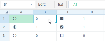
If you need to get the state of a checkbox or a radio button, you can apply the getCellValue method to the necessary cell:

const isChecked = $$("ssheet").getCellValue(1, 1, false); 
// -> 1 - checked, 0 - unchecked

Another way to check the state is to refer to the cell with the necessary checkbox or radio button via the setCellValue method in a different cell. You will get 1, if the checkbox/radio button is marked and 0, if it isn't marked. For example:

// getting the state of the radio button from the cell A1 in the cell B1
$$("ssheet").setCellValue(1,2,"=A1");

You can also specify a more complex condition, e.g. to use some text that will be rendered in the resulting cell, depending on the state of the checkbox or radio button in the referred cell:

// getting the state of the radio button from the cell A2 in the cell A5
$$("ssheet").setCellValue(5,1,"=IF(A2,\"A2 marked\", \"A2 is not marked\")");

Filtering Cells Values

Setting a filter in a cell

You can set a filter inside of a cell. This is how you can add a filter from the UI:

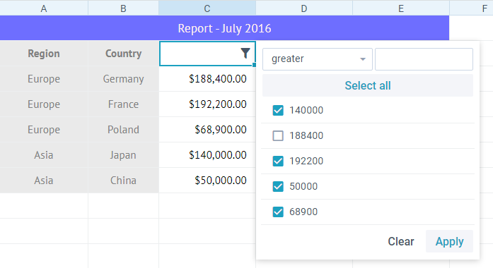
The setCellFilter method will help you to set a filter via the API. You need to pass the following parameters to this method:

• rowId - (number) the row id
• columnId - (number) the column id
• filterObject - (object) the filter object that can have the following properties:
  • options (string, array) - a range of cells references the values of which will be filtered or an array of filter options
  • mode (string) - filter mode. If not specified takes the type from the first not empty cell in the column
  • value (object) - sets a filter value. Call the filterSpreadSheet to invoke the filter.
  • lastRow (number) -a cell where the filtering will stop. If not specified, filtration will stop at the first empty cell that comes up
• page - (string) optional, the name of the sheet

// an array of options
$$("ss1").setCellFilter(1, 2, {
    options: ["", "Europe", "Asia", "America"],
    mode: "text",
    value: values,
    lastRow: 3
}, "Sheet1");
 
// a range of cells references
$$("ss1").setCellFilter(2, 2, {
    options: "B3:B7",
    mode: "text",
    value: values,
    lastRow: 3
}, "Sheet1");

It is possible to specify a range of cells references the values of which will be filtered or an array of filter options as a third parameter instead of the filter object:

$$("ssheet").setCellFilter(2,1, ["", "Europe", "Asia", "America"] );
 
// or
$$("ssheet").setCellFilter(2,2, "B3:B7");

Related sample:  Filters

Getting the cell filter

To get a filter set in a cell, make use of the getCellFilter method. It takes the following parameters:

• row - (number) the row id
• column - (number) the column id
• page - (string) optional, the name of the sheet

and returns an object with a set of options and the IDs of the row and column:

• options - (string/array) a string or an array with the filter option(s)
• row - (number) the ID of the row
• column - (number) the ID of the column

Check the example below:

$$("ssheet").getCellFilter(2, 1, "Sheet1"); 
// -> { options: Array(4), row: 2, column: 1 }

Sorting Cells Values

SpreadSheet allows you to sort values within a selected or specified range of cells via the sortRange method. You can pass two optional parameters to it:

• range - (string) optional, the range of cells that should be sorted, null to sort the selected range. Note that sorting of multiple ranges is not supported
• config - (string|object) optional, the sorting direction: "asc" or "desc" ("asc" by default) or an object for configuring multi-column sort

// sorts the specified range in the default ("asc") order
$$("ssheet").sortRange("B2:B4");
// sorts the specified range in the descending order
$$("ssheet").sortRange("B2:B4", "desc");
// sorts the selected range in the descending order
$$("ssheet").sortRange(null,"desc");

Related sample:  Sorting

To configure multi-column sort, pass an object as the config parameter:

// sorts the range A1:C10 by column B (ascending), then by column C (descending)
$$("ssheet").sortRange("A1:C10", {
    hasHeaders: true,
    levels: [
        { column: "B", direction: "asc" },
        { column: "C", direction: "desc" }
    ]
});

The object for configuring multi-column sort in the config parameter has the following structure:

{
    hasHeaders: boolean; 
    levels: [
        { column: string | number, direction: string },
        ...
    ]
}

The default values of the config set as an object are:

{
    hasHeaders: false,
    levels: [
        { 
            column: range.start.column, // id of the first column of the sorted range
            direction: "asc" 
        }
    ]
}

where:

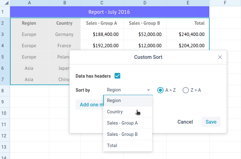
• hasHeaders - (boolean) false by default. The code representation of the checkbox in the Custom Sort dialogue:

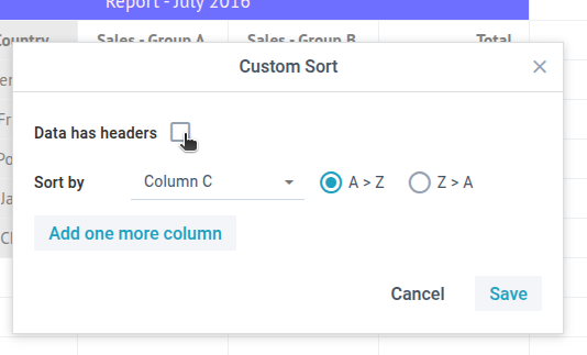
If true, the first row of the selected range of cells would behave as the headers and the names of these headers will be displayed in the Sort by dropdown list instead of plain Column A, B, C:

• levels - (array) represents an array of columns' objects to sort the data at. Each column object includes:
  • column - (string|number) required, the column ID as a string (e.g.: "A", "AA" or "X", etc.) or a number (1, 2, etc.)
  • direction - (string) optional, the sorting direction: "asc" or "desc" ("asc" by default)

The order of levels matters. This is the order in which column sort config is going to be applied to data. The 2nd+ levels are so-called tiebreakers and applied only if the previous comparison ended in a tie (both equal).

Validating Cells Content

There is a possibility to add a validation rule for the content of a cell. A validation rule can be added to a cell through the SpreadSheet interface, namely: via the Validation button on the Toolbar:

or via the Menu or Context Menu options. A click on the "Add data validation" option will open a dialog popup:

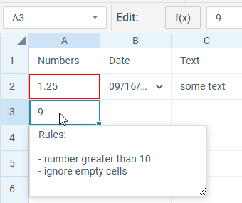
This popup contains a set of validation rule types and their attrubutes. After a user adds a validation rule to a cell, a click on it will call a textarea with the rule details:

Each validation rule includes a number of parameters:

• the row id
• the column id
• the validation rule
• the number of the page where the cell is placed

A validation rule can have one of the following types:

• "any" (a cell can have any content)
• "date"
• "number"
• "text"
• "textLength"
• "range" (to validate data among a range of cells)

Depending on the type of the rule, it can have the following attributes:

• Integers only - (for the number type) for accepting only integer numbers
• Ignore empty - to ignore/ not ignore empty cells
• Condition - the condition that will be applied. Depending on the rule type, may include the following values:
  • greater
  • less
  • greater or equal
  • less or equal
  • equal
  • not equal
  • between
  • not between
  • contains
  • not contains
  • begins with
  • not begins with
  • ends with
  • not ends with
• Value - a value or an array of two values (for the rules like "between/not between") that should be compared to the value of the specified cell
• Input message - a popup with the text specified in this property will be shown on selection of a cell
• Error handle - the way of handling an error (in the corresponding confirm box):
  • "stop" - doesn't allow setting an incorrect value
  • "warning" - allows cancelling the set value
  • "information" - an box informing that the value is not valid
• Error title - the header of the confirm box with an error
• Error message - the text of the confirm box with an error

Validation API

You can specify validation rules for a cell directly in a data source.

For this purpose, use the validation module of the data object. You can specify a set of validation rules in one array:

data.validation = [
    [
        "2",
        "1",
        {
            "type": "number",
            "integer": 1,
            "empty": 1,
            "condition": "greater",
            "value": "0",
            "inputMessage": "Rules:\n\n- integer greater than 0\n- include empty",
            "errorHandle": "info",
            "errorTitle": "Incorrect data!",
            "errorMessage": "Should be integer greater than 0!"
        }
    ],
    [
        "2",
        "2",
        {
            "type": "date",
            "empty": 0,
            "condition": "greater",
            "value": "45292",
            "inputMessage": "Rules:\n\n- date after 01/01/2024\n- exclude empty",
            "errorHandle": "stop",
            "errorTitle": "Incorrect data!",
            "errorMessage": "Should be date after 01/01/2024!"
        }
    ]
];

The validation collection also allows you to manage validation rules:

• add/remove validation rules
• get validation rules of the specified cell
• add/remove highlighting for cells with applied validation rules

Add a validation rule to a cell

You can add a validation rule to a cell by using the validation.add(row, column, rule, page) method. It takes the following parameters:

• row (number) - the row ID
• column (number) - the column ID
• rule (object) - the validation rule. Has the following attributes:
  • type (string) - the validation criteria. It can be: "any" (a cell can have any content), "date", "number", "text", "textLength", "range" (to validate data among a cells range)
  • integer (boolean) - (for the number type only) true for accepting integer numbers only
  • ignoreEmpty (boolean) - true to ignore/ not ignore empty cells
  • condition (string) - a condition for validation
  • value (string/array) - a value or an array of two values (for the rules like "between/not between") that should be compared to the value of the specified cell
  • inputMessage (string) - a popup with the text specified in this property will be shown on selection of a cell
  • errorHandle (string) - the way of handling an error (in the corresponding confirm box):
    • "stop" - doesn't allow setting an incorrect value
    • "warning" - allows cancelling the set value
    • "information" - an box informing that the value is not valid
  • errorTitle (string) - the header of the confirm box with an error
  • errorMessage (string) - the text of the confirm box with an error
• page - (string) optional, the name of the sheet. If not specified, applies the method to the current sheet

// adding a validation rule for the cell B3 of the page 2
$$("ssheet").validation.add(
    3, 
    2, 
    {
      "type": "number",
      "integer": 1,
      "empty": 1,
      "condition": "greater",
      "value": "0",
      "inputMessage": "Rules:\n\n- integer greater than 0\n- include empty",
      "errorHandle": "info",
      "errorTitle": "Incorrect data!",
      "errorMessage": "Should be integer greater than 0!"
    }, 
    2
);

Remove a validation rule from a cell

To remove the applied validation rule from a cell, use the validation.remove(row, column, page) method. It takes the following parameters:

• row (number) - the row ID
• column (number) - the column ID
• page - (string) optional, the name of the sheet. If not specified, applies the method to the current sheet

// removing the validation rule from the cell B3 on page 2
$$("ssheet").validation.remove(3, 2, "Sheet1");

Get the validation rule of the specified cell

To get the validation rule applied to a cell, use the validation.get(row, column, page) method. It takes the following parameters:

• row (number) - the row ID
• column (number) - the column ID
• page - (string) optional, the name of the sheet. If not specified, applies the method to the current sheet

// getting the validation rule of the cell B3 on page 2
$$("ssheet").validation.get(3, 2, "Sheet1");

Add/remove highlighting of cells with validation rules

You can add/remove highlighting to/from a cell with applied validation rules. Use the validation.highlight(state, page) method. It takes the following parameters:

• state (boolean/"toggle") - true if highlighting for cells with validation rules is enabled
• page - (string) optional, the name of the sheet. If not specified, applies the method to the current sheet

// removing highlighting from cells with applied validation rules from the page 2
$$("ssheet").validation.highlight(false, "Sheet1");

Adding Sparklines into a Cell

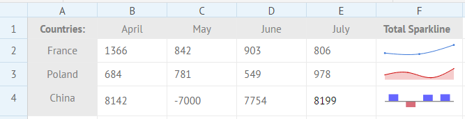
You can add a small chart into a cell to display tendencies of data values changing in a range of cells.

To insert a sparkline inside of a cell, use the addSparkline method with the following parameters:

• rowId - (number) the row id
• columnId - (number) the column id
• config - (object) the sparkline configuration that have the properties below:
  • type - (string) the type of an added sparkline
  • data - (string) the range of cells the values of which will be displayed in the sparkline
  • color - (string) the color of a sparkline either in a hex format or as a color name
  • negativeColor - (string) the color of a negative value for a Bar sparkline
• page - (string) optional, the name of the sheet. If not specified, the method is applied to the current sheet

$$("ssheet").addSparkline(rowId, columnId, config, page);

Let's insert a blue sparkline of the Line type into the cell E5. The passed parameters will be as follows:

$$("ssheet").addSparkline(5, 5, {type:"line", range:"B4:E4", color:"#6666FF"});

Related sample:  Adding sparklines

Adding Image in a Cell

You can add an image into a cell to illustrate data in the spreadsheet.

To insert an image into a cell, use the addImage method. You need to pass the following parameters to this method:

• rowId - (number) the row id
• columnId - (number) the column id
• url - (string) the URL of an image
• page - (string) optional, the name of the sheet. If not specified, the method is applied to the current sheet

$$("ssheet").addImage(2,3, "http://docs.webix.com/media/desktop/image.png", "Sheet1");

Related sample:  Adding images

Adding Comments into Cells

There is a possibility to add a comment into a certain cell of SpreadSheet.

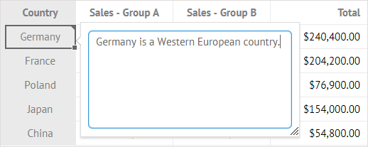
Use the add() method of the comments object. It takes three parameters:

• rowId - (number) the row id
• columnId - (number) the column id
• comment - (string) the text of a comment
• page - (string) optional, the name of the sheet. If not specified, the method is applied to the current sheet

// adding a comment into the cell B3
$$("ssheet").comments.add(3, 2, "text", "Sheet1");

The API of the comments object also makes it possible to get a comment of a particular cell or to delete a comment that is no longer needed:

// getting a comment for the cell B3 of Sheet1
$$("ssheet").comments.get(3, 2, "Sheet1");
 
// removing a comment from the cell B3 of Sheet1
$$("ssheet").comments.remove(3, 2, "Sheet1");

Using Placeholders

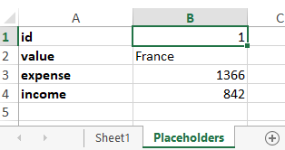
You can specify what data will be displayed in the SpreadSheet cells by using placeholders.

A placeholder is an object with data properties which can be set as SpreadSheet values. To define a placeholder use the setPlaceholder method:

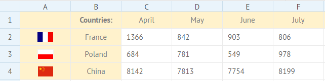
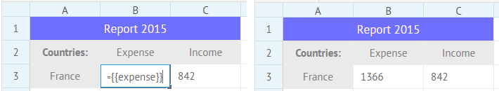
$$("ssheet").setPlaceholder({value:"France", expense:1366, income:842});

If the placeholder is a string, you need to provide the value as the second parameter:

$$("ssheet").setPlaceholder("expense", 1366);

Pay attention that the names of placeholders can't contain the following special characters:

• Spaces
• Operators: + - * / = > < ~ ? !
• Curly brackets, parentheses, quotes, double quotes: { } ( ) " '
• Other special characters, including: , | \ : ; @ % ^ &

It is recommended to use underscores instead of spaces in the names of placeholders that contain several words, for example: "my_name".

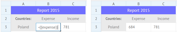
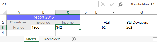
To specify a placeholder's property in a cell instead of a value, use the ={{property}} construction. For example, for cells with the "expense" values you should specify placeholders as "={{expense}}".

If you specify a new placeholder for a SpreadSheet, values of all cells where properties of this placeholder are defined will be updated.

$$("ssheet").setPlaceholder({value:"Poland", expense:684, income:781});

Related sample:  Placeholders

Adding placeholders on an extra sheet on Excel export

Take notice that while exporting Spreadsheet data to Excel, placeholders are replaced with their values. For example, if you have a placeholder =A1+{{value}}, where value is 10, the formula in the cell will be replaced with the expression =A1+10.

However, you can put all the placeholders to a separate sheet and refer to them as =A1+Placeholders!B1 (where "Placeholders" is the name of the sheet with placeholders). This approach allows you to edit them in the Excel file.

Here is an example of an Excel file with exported spreadsheet data and placeholders:

Related sample:  Extra Placeholder Sheet on Excel Export

Applying Borders to Cells

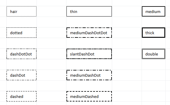
SpreadSheet provides all border types available in Excel:

• hair
• dotted
• dashDotDot
• dashDot
• dashed
• thin
• mediumDashDotDot
• slantDashDot
• mediumDashDot
• mediumDashed
• medium
• thick
• double

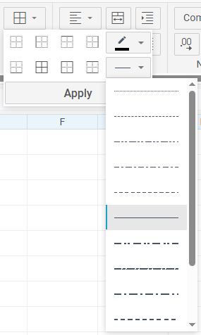
To choose a border type, open the Borders popup in the toolbar and use the Border line type control.

The borderCollapse configuration property controls how Spreadsheet renders cell borders.

There are two modes of applying borders to cells:

• borderCollapse: false - (default) each cell has its own borders

• borderCollapse: true - borders are shared between adjacent cells in the Excel-like style

In this mode, the border between two neighboring cells is owned by the right cell (for vertical borders) or the bottom cell (for horizontal borders). As an exception, the top and left borders can be set on the starting (top-left) cell of a bordered range.

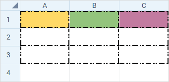
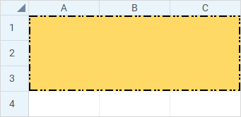
Merging cells

Spreadsheet allows merging adjacent cells into a single cell via the toolbar, menu, or the API. The merged cell displays the value and style of the top-left cell of the range.

In the image below the cells of the first row are merged:

Merging cells via API

To merge cells via the API, use the combineCells method. It takes an optional range object and an optional sheet name:

$$("ssheet").combineCells({cell:{row:4, column:5}, x:2, y:2}, "Sheet1");

The method takes the following parameters:

• range - (object) optional, the range of cells to merge. The object includes:
  • cell - (object) the id of the cell that starts the range:
    • row - (number) the row index of the cell
    • column - (number) the column index of the cell
  • x - (number) the number of cells to merge horizontally
  • y - (number) the number of cells to merge vertically
• page - (string) optional, the name of the sheet

If no range is specified, Spreadsheet merges the currently selected cells.

Splitting merged cells

To split merged cells, use the splitCell method:

$$("ssheet").splitCell(4, 5, "Sheet1");

The method takes the following parameters:

• row - (number) the row index of the cell the span starts with
• column - (number) the column index of the cell the span starts with
• page - (string) optional, the name of the sheet

Getting cell span

To check whether a cell has a span, use the getSpan method:

const span = $$("ssheet").getSpan(1, 1);
// returns [1, 1, 5, 1]

The method takes the following parameters:

• row - (number) the row index of the cell
• column - (number) the column index of the cell
• page - (string) optional, the name of the sheet

The method returns an array in the same format as the spans field in the data:

• the row index that starts the span
• the column index that starts the span
• the number of columns in the span
• the number of rows in the span

If the cell has no span, the method returns undefined.

Styles merging behavior

• Spreadsheet applies the style of the top-left cell to all merged cells.
• When setting styles via the toolbar or menu, Spreadsheet applies them to all cells in the merge. To set a style for a single cell individually, use the API.
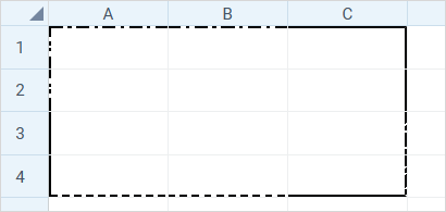
• If the cells have borders before merging, Spreadsheet removes the inner borders and applies the outer borders based on the borders set on the perimeter.

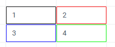
For example:

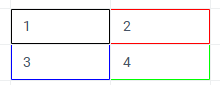
On merging the cells, Spreadsheet applies styling as shown below:

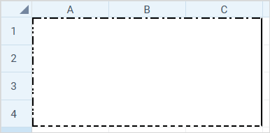
• Cell borders can be solid or dashed. If you apply mixed solid and dashed borders to cells in a range, Spreadsheet uses the first border type it encounters during merging.

For example:

The result of merging cells with different border types is the following:

Importing merged cells with borders

Set sheetStubs:true if you want to import an Excel file that contains merged cells with borders. It imports the styles of empty cells under the span, so that all cells in the merged range have borders. Otherwise, only the top-left cell of the merged range will have borders.

Back to top